I frequently need to use non-linear regression in Grasshopper, usually for interpolating data points on a 2D map. For example, if I have real data set for rainfall that includes latitude, longitude, and annual rainfall, I might want a non-linear regression model that allows me to pick any coordinates and interpolate the rainfall data for that point based on the points around it. I frequently use the Non-Linear Regression component in Proving Ground’s LunchBoxML toolkit, but there are several occasions in which it’s challenging to set the right parameters to get the fit that I had in mind. This happens when the first two variables are so small or large (like with latitude and longitude) that the default sigma and complexity values in the LunchBoxML component are too far out of range to work. Sometimes the data is smooth in some places (like East Coast rainfall) and complex in other places (like Rocky Mountain rainfall) and there’s no good compromise for a best fit.
I’m sure there’s a proper way to get it to work, but I often use a simpler method instead. This script gives each test point a value based on the average of its closest points, then smooths out the data based on a confidence score.
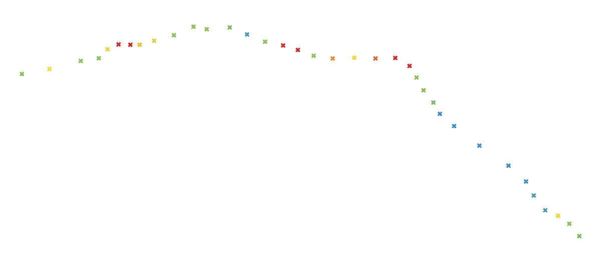
For example, this is a data set of illuminance along a path. Red indicates brighter, blue indicates darker.
The first part of the script draws a bounding box around the known data points, and creates a test grid evenly across the box.
Each test point is given a value based on the average of its three closest data points. This creates an accurate smoothing along the path, but also creates unrealistic fault lines further from the path.
Each test point is given a confidence score based on how close it is to a real data point. High confidence points stay close to their first estimate, low confidence points return a value closest to the mean value of all data points.
This results in a reasonably smooth interpolation that doesn’t over-smooth the high-confidence data points along the path.


